Logistic regression and support vector machine
Classification falls in the category of supervised learning. A set of training data \(\left(x^{(i)}, y^{(i)}\right)\) is given where \(x^{(i)}\in \mathbb{R}^N\) is the feature vector and \(y^{(i)}\) is its label.
For simplicity, let’s assume that the data points are linearly separable and there are only two categories, i.e., \(y^{(i)}\) is either 0 or 1.
The rationale behind both logistic regression (LR) and support vector machine (SVM) is to find a line (2D) or hyperplane to separate the data points into two groups, as seen in Fig. 1. The hyperplane can be parametrized as \(z\equiv w^Tx+b=0\) where the weights \(w\) and bias \(b\) are the unknown parameters. Since more than one plane may serve the purpose, some kind of optimality needs to be introduced. Roughly speaking, SVM maximizes the distance from the separation plane to the closest points whereas LR maximizes the distance from the plane to all points.

Figure 1. Hyperplanes \(H_2\) and \(H_3\) separate the data points successfully.
Logistic regression
LR is a probabilistic model. The likelihood of the label is explicitly specified as
\[p(y=1|x) = \sigma (z)\]where
\[\sigma(z) \equiv \frac{1}{1+e^{-z}}\]Looking at Fig. 2, any point with \(z>0\) will have over 50% chance to have label 1. Similarly, any point with \(z<0\) is more likely to have label 0. Note that the distance of the data point to the separation plane is proportional to the numerical value of \(|z|\). The choice of sigmoid function thus reflects the intuition that the farther away from the separation plane the more confident we are about the label assignment.

Figure 2. Simgoid function \(\sigma(z)\).
One may wonder why we don’t simply label the point as 1 if its \(z^{(i)}>0\). In other words, to use heaviside step function for \(p(y=1|x)\). It works too! The corresponding model is called perceptron, which was proposed by Frank Rosenblatt in 1957. I don’t have convincing argument why LR is better than perceptron. One obvious difference is that the LR model is differentiable. But it’s not very clear why continuity at one point helps.
To get \(w\) and \(b\) in LR, one can solve a minimization problem. For example, the cost function could take the form
\[C(w, b) = \sum_i \left( y^{(i)} - \sigma(z^{(i)})\right)^2\]Intuitively, with label 0, \(\sigma(z)\) should be small and with label 1, \(\sigma(z)\) should be big. This quadratic cost function turns out to be a bad choice because its derivative to \(w\) and \(b\) is likely to vanish as minimization proceeds. For example,
\[\partial_b C = - \sum_i\left( y^{(i)} - \sigma(z^{(i)})\right)\sigma'(z^{(i)})\]As seen from Fig. 2, the derivative of the sigmoid function is small in most places. Also, as the cost function is minimized, the model fit on the training data gets better and unfortunately, the derivative of the quadratic cost function also gets smaller.
To avoid this vanishing gradient problem, one can use the cross entropy cost function
\[C = -\sum_i y^{(i)}\log(\sigma(z^{(i)}))+ (1-y^{(i)})\log (1-\sigma(z^{(i)}))\]One can easily check \(C\) at least intuitively make sense since \(1\log1=0\) and \(0\log0=0\).
Now the derivative becomes
\[\begin{align} \partial_b C =& \sum_i \sigma(z^{(i)})- y^{(i)} \\ \partial_{w_k} C =& \sum_i x_k^{(i)}\left(\sigma(z^{(i)})-y^{(i)} \right) \end{align}\]where we have used \begin{align} \sigma’(z) =\sigma(z)(1-\sigma(z)). \end{align}
It thus gets rid of the \(\sigma'(z)\) part.
With the derivatives of the cost function, gradient descent can be used to solve the minimization problem. In practice, it is common to add a regularization term (say L2) to the cost function to make the model more well-determined.
There is a probabilistic interpretation of the cross entropy cost function. Our binary classification problem can be considered as a Bernoulli distribution over two labels. The probability of a data point to have label \(y\) is given by
\[P(y|x) = \sigma(x)^y (1-\sigma(x))^{1-y}\]Thus the likelihood of the training data to have the correct label is
\[L(w, b) = \Pi_i P(y^{(i)}|x^{(i)})\]and the cross entropy cost function is the log likelihood function \(C= \log L(w,b)\).
Finally I would like to point out that the cross entropy cost function tries to achieve the same goal as the quadratic cost function: the \(\sigma(z^{(i)})\) should be as close to 0 or 1 as possible. In other words, \(|z^{(i)}|\) should be as big as possible, or geometrically, the points should be as far away from the separation plane as possible. Since the total cost function is a summation over all the data points, LR aims at maximizing the total ‘distance’ from the separation plane to all the data points.
Support vector machine
SVM is a non-probabilistic model of classification. It has a clear geometric meaning that the optimal hyperplane \(z=0\) has the largest distance to the nearest training data, as seen in Fig. 1.
Recall that any plane that is parallel to the separation plane can be parametrized by \(z=w^Tx+b\neq0\). The weight vector \(w\) is perpendicular to the plane and serves as normal vector. When \(w\) is given, the separation between the two data sets with different labels along \(w\) direction is determined. Let’s assume \(x^{(A)}\) and \(x^{(B)}\) are the two points with different labels that are closest to the separation plane. They are the so-called support vectors. By requiring
\[\begin{align} w^Tx^{(A)} + b =& 1 \\ w^Tx^{(B)} + b =& -1,\end{align}\]the distance between \(x^{(A)}\) and \(x^{(B)}\) along \(w\) direction is then given by \(\frac{2}{\|w\|}\). Note that although \(z=0\) uniquely specifies the separation plane, it does not uniquely specify \(w\) and \(b\) due to their scale ambiguity. \(z^{(A)}=1\) fixes their scale. Furthermore, \(z^{(B)}=-1\) does not place extra constraint since the separation plane is right in the middle of the two planes \(z^{(A)}=1\) and \(z^{(B)}=-1\).
Another consequence of these two equations is
\[\begin{align} z^{(i)}\ge1, & \quad \text{if } y^{(i)} = 1 \\ z^{(i)}\le1, & \quad \text{if } y^{(i)} = 0 \end{align}\]for all data points. It is thus more convenient to change the label 0 to -1 for notational convenience. Then the two inequalities can be combined into one:
\[y^{(i)} z^{(i)}\ge 1.\]Thus the optimal separation plane is the solution of the following optimization problem
\[\max\frac{2}{\|w\|}, \quad s.t.\quad y^{(i)} z^{(i)}\ge 1,\]or equivalently
\[\min\|w\|, \quad s.t. \quad y^{(i)} z^{(i)}\ge 1.\]It is a convex optimization problem and can be efficiently solved using primal dual method. Further complications of SVM can be found in this post.
Their differences
As mentioned above, SVM cares only about the points closest to the separation plane whereas LR cares about all the points. Thus their results in general differ. With symmetrical data, as in Fig. 3, both methods give the same result. With an extra data point, as in Fig. 4, the LR result changes whereas the SVM result remains the same.
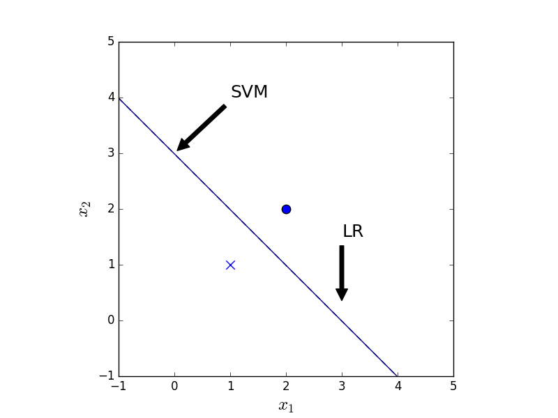
Figure 3. The classification result of LR (dashed) and SVM (solid) given 2 data points.
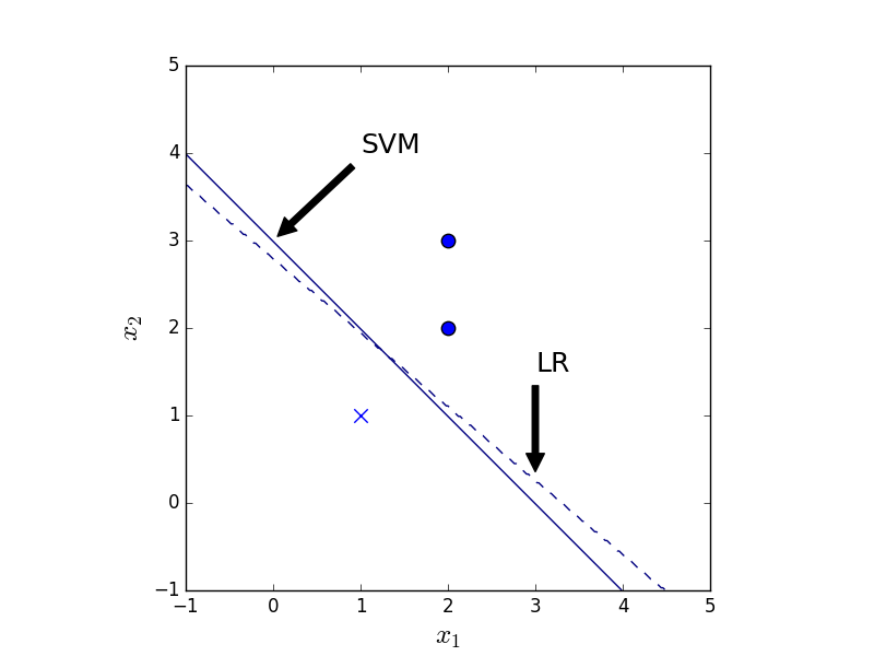
Figure 4. The classification result of LR (dashed) and SVM (solid) given 3 data points.
As for which method is better, it may depend on the problem. For example, what kind of outlier does one expect in the data set. In real life, data might not even be linearly separable. In that case, kernel SVM with soft margin will be an option. In terms of computation cost, LR is way faster than SVM.
appendix
The code to generate Fig. 4 is as follows.
The parameter C controls the size of regularization.
By setting C to be large, the regularization is effectively turned off.
from sklearn.linear_model import LogisticRegression
from sklearn.svm import SVC
import numpy as np
import matplotlib.pyplot as plt

X = np.array([[1, 1], [2, 2], [2,3]])
y = np.array([0, 1, 1])
lr = LogisticRegression(C=1e10, penalty="l2",
                    random_state=0, verbose=True)
lr.fit(X, y)
svm = SVC(kernel='linear', C=1e10,
                    random_state=0, verbose=True)
svm.fit(X, y)

# make plot
fig = plt.figure(frameon=False)
x1_min, x1_max = -1, 5
x2_min, x2_max = -1, 5
h = 0.02
xx1, xx2 = np.meshgrid(np.arange(x1_min, x1_max, h),
                    np.arange(x2_min, x2_max, h))
# SVM
Z = svm.predict((np.array([xx1.ravel(), xx2.ravel()]).T))
Z = Z.reshape(xx1.shape)
plt.axes().annotate('SVM', xy=(0, 3), xytext=(1, 4),
            arrowprops=dict(facecolor='black', shrink=0.05),
                            size=18)
plt.contour(xx1, xx2, Z, levels=[0.5], linestyles='solid')
# LR
Z = lr.predict((np.array([xx1.ravel(), xx2.ravel()]).T))
Z = Z.reshape(xx1.shape)
plt.axes().annotate('LR', xy=(3, 0.3), xytext=(3, 1.5),
            arrowprops=dict(facecolor='black', shrink=0.05),
                            size=18)
plt.contour(xx1, xx2, Z, levels=[0.5], linestyles='dashed')

plt.scatter(X[0,0], X[0, 1], marker='x', s=80)
plt.scatter(X[1,0], X[1, 1], marker='o', s=80)
plt.scatter(X[2,0], X[2, 1], marker='o', s=80)
plt.xlabel('$x_1$', fontsize=18)
plt.ylabel('$x_2$', fontsize=18)
plt.xlim(x1_min, x1_max)
plt.ylim(x1_min, x1_max)
plt.axes().set_aspect('equal')
plt.show()


