Naive Bayes classifier
introduction
This post is a tutorial on naive Bayes classifier. As you will see, the underlying idea is quite natural and intuitive. To be concrete, let’s compare apples and oranges.
I will consider three features for the fruits:
- weight (\(x_1\)): either continuous or binary (greater or less than a cutoff)
- color (\(x_2\)): red / green / orange
- tenderness (\(x_3\)): soft / hard
In probability theory, the treatments for continuous and discrete variables are slightly different. If you want to be more relaxed, think of weight as a binary feature.
The problem can be formulated as follows. We already have a lot of apples and oranges in stock and have recorded the features \((x_1, x_2, x_3)\) for each of them. Now a new fruit comes in and we need to decide whether it is an apple or an orange.
To make the notation simple, let’s define a class label \(y\) and
- apple: \(y=0\)
- orange: \(y=1\)
More on notations:
- I will also write \((\mathbf x)\) to denote \((x_1, x_2, x_3)\).
- To distinguish features from a specific fruit, I will use superscript, e.g., \(\left(x_1^{(k)}, x_2^{(k)}, x_3^{(k)}\right)\).
- I will NOT use upper-case letters for random variables and lower-case letters for values. Hopefully the context will make the meaning clear. If not, please drop me a comment.
brain storming
It may be very tempting to use the following approach:
- find a few fruits in stock that resemble the new one
- do a majority vote on them
It is surely a valid and very practical approach. It is essentially the k-nearest neighobors algorithm. But for the sake of this post, let’s think of something else.
more brain storming
To me, it’s also very tempting to think of the following
- calculate the distributions for individual features using fruits in stock
- check where the new fruit stands in these distributions and then decide
Basically the first step estimates \(P(x_i|y)\) using existing data and the second step requires some judgement. In the figure below, I generated some fictitious \(P(x_i|y)\).
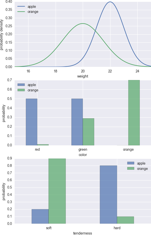
Now suppose the new fruit is heavy, green and hard. Based on the plots, we can confidently conclude that it is an apple.
digression No. 1
You may wonder why do we estimate \(P(x_i|y)\), instead of \(P(\mathbf x|y)\). Indeed, it makes more sense to use the latter to make predictions on the new fruit and it is essentially the maximum likelihood method.
However, there are several reasons against it:
- My little brain prefers to think about single-variable, rather than multi-variable functions
- With a given dataset (sample size), it’s easier and much more reliable to estimate single-variable distributions.
Of course the second reason is a more practically limiting one. With the curse of dimensionality, accurate estimation of the joint probability distribution quickly becomes difficult as the number of features increases. To make things worse, the features may be continuous variables, and we may not have good prior information about the functional form of their distributions. In these cases, estimating \(P(\mathbf x|y)\) from a dataset becomes mission impossible.
digression No. 2
What if the new fruit is medium weight, red and soft?
These unpleasant situations need to be handled by mathematical formula, instead of human eyeballing. For me, it’s very tempting to simply multiply the single-feature conditional probabilities together, i.e.,
\[P(x_1^{\text{new}}|y)P(x_2^{\text{new}}|y)P(x_3^{\text{new}}|y)\]Then we compare the \(y=1\) and \(y=0\) cases and decide. Hopefully this approach will vaguely make some sense to you too.
What is the rationale behind this hand-waving approach? For me, I am secretly hoping that the following ‘equation’ is true.
\[P(x_1, x_2, x_3|y) \overset{?}= P(x_1|y)P(x_2|y)P(x_3|y)\]In other words, I was hoping that \(P(\mathbf x|y)\) could be calculated cheaply from \(P(x_i|y)\).
Clearly it cannot be true in general, as can be seen from the following equation:
\[P(x_1, x_2, x_3) \neq P(x_1)P(x_2)P(x_3)\]The above inequality becomes equality only when \(x_i\) are independent random variables.
Does the notion of independence exist in our conditioned situation? Unfortunately there is no guarantee of the conditional independence among the features. Thus in general our ‘equation’ with question mark does not hold and we can at best think of \(P(x_1^{\text{new}}|y)P(x_2^{\text{new}}|y)P(x_3^{\text{new}}|y)\) as a hand-waving approximation of \(P({\mathbf x}^\text{new}|y)\).
digression No. 3
Suppose we somehow managed to get \(P(\mathbf x|y)\) from our stock, or maybe we are satisfied with the hand-waving approximation of it from the digression No. 2. Now some trustworthy person comes in and provides an extra piece of information: there is 1 billion apples and 1 million oranges on this planet.
Should we care?
It’s a personal question about whether one should take the frequentist or the Bayesian view. Or equivalently, use maximum likelihood estimation or maximum a posteriori (MAP) estimation.
In our problem, it is hard to judge whether the new fruit actually comes from a uniform sampling scheme of the planet’s apple/orange reservoir. In some cases, you may have a more convincing argument to use MAP.
Anyways, if we decide to add in the prior information, then we can compute
\[P(y)P({\mathbf x}^\text{new}|y)\]and then decide whether \(y=0\) or \(y=1\). The extra factor of \(P(y)\) is able to change our prediction. Thus you can get help (cheat) from it.
If extra prior information is not provided from elsewhere, \(P(y)\) can be estimated from our stock as well.
brief summary before we proceed
So far, combining all three digressions, what we have is a hand-waving quantity
\[P(y)P(x_1^\text{new}|y)P(x_2^\text{new}|y)P(x_3^\text{new}|y)\]It is actually the naive Bayes classifier already.
a more formal treatment
For our classification problem, what we really want is \(P(y|\mathbf x)\), the probability of the class label conditioned on the features.
Using the Bayes’ rule, we have
\[P(y|\mathbf x) = \frac{P(y)P(\mathbf x|y)}{P(\mathbf x)}\]In plain English, it can be read as
\[\text{posterior} = \frac{\text{prior}\times\text{likelihood}}{\text{evidence}}\]Using the chain rule of probability to further simplify \(P(\mathbf x|y)\), we get
\[P(y|\mathbf x) = \frac{P(y)}{P(\mathbf x)}P(x_1|y)P(x_2|y, x_1)P(x_3|y, x_1, x_2)\]Now it’s clear what it takes to get \(P(y|\mathbf x)\):
- the prior \(P(y)\)
- the likelihood of each feature conditioned on class label and other features
- the evidence \(P(\mathbf x)\) is not relevant since it is a common denominator
Comparing to the formula in the previous section, it is then clear what the naive Bayes classifier is assuming:
\[P(x_2|y,x_1) \simeq P(x_2|y) \\ P(x_3|y,x_1,x_2) \simeq P(x_3|y)\]In other words, we are assuming the conditional independence between the features, as alluded in the digression No. 2.
summary
I hope that you have enjoyed the reading and found naive Bayes an intuitive idea. In short, it is a poor man’s MAP estimation with conditional independence assumption.
appendix
The code to generate the plot is as follows
import matplotlib.pyplot as plt
import seaborn as sns
import pandas as pd
import numpy as np
import matplotlib.mlab as mlab

# prepare the canvas
fig = plt.figure(figsize=(7,11))
ax1 = fig.add_subplot(3,1,1)
ax2 = fig.add_subplot(3,1,2)
ax3 = fig.add_subplot(3,1,3)

# draw two gaussians
mu1, mu2 = 22, 20
s1, s2 = 1, 1.5
x = np.linspace(15,25, 100)
ax1.plot(x, mlab.normpdf(x, mu1, s1), label='apple')
ax1.plot(x, mlab.normpdf(x, mu2, s2), label='orange')
ax1.set(xlim=(15,25), xlabel='weight', ylabel='probability density')
ax1.legend(loc='upper left')

# draw color
color = pd.DataFrame({'apple':[0.5, 0.5, 0], 'orange':[0.01, 0.29, 0.7]},
                index=['red', 'green', 'orange'])
color.plot(kind='bar', ax=ax2, rot=0, alpha=0.7)
ax2.set(xlabel='color', ylabel='probability')

# draw tenderness
tender = pd.DataFrame({'apple':[0.2, 0.8],'orange':[0.9,0.1]},
                index=['soft', 'hard'])
tender.plot(kind='bar', ax=ax3, rot=0, alpha=0.7)
ax3.set(xlabel='tenderness', ylabel='probability')

#sns.plt.show()
fig.savefig('out.png', bbox_inches='tight', pad_inches=0)


