Tree-based classifiers
Tree-based classifiers are commonly used in practice. Their pros and cons are as follows.
- pros
- relatively fast to train
- able to achieve very good performance
- able to classify data that are NOT linearly separable
- somewhat easy to interpret the results
- able to treat categorical features almost out-of-box
- cons
- somewhat unstable (of high variance, somewhat difficult to generalize)
In this post, I will introduce four models
Decision tree is the basic building block of all tree-based classifiers. The later three classifiers average over many trees for better result. In machine learning jargon, they are ensemble methods that build strong learner out of weak learners.
In practice, you probably don’t want to use decision tree due to its instability. Both random forest and boosted trees can provide good result almost out-of-box without feature engineering. I have seen some case studies in books saying that boosted trees may be slightly better than random forest.
For simplicity, I will use binary classification problem as example and binary decision tree as building block in this post. The class labels are black and white, or \(Y\in\{0, 1\}\) and the features are two real valued variables \((x_1, x_2)\). One set of training data is shown in Figure 1.
Figure 1. Black and white dots to be classified. Try the update button.
Personally, I find the tree-based classifiers less natural to think of than the more ‘geometric’ methods such as logistic regression or support vector machine. They deviate from my comfortable zone of linear algebra + calculus, and contain some degree of messiness and magic which I will comment on later.
decision tree
The decision tree classifier uses a series of decisions to determine the class label. In the case of binary decision trees, one raises yes/no questions, as shown in Figure 2. It is similar to the game Botticelli.
The root node and internal nodes of the tree are the decisions to be made, whereas the terminal nodes (leaves) are the class labels.
Figure 2. This decision tree generates the decision boundaries in Figure 1.
Geometrically, these yes/no questions partition the feature space into rectangles (boxes) for data with different labels. Try the update button in Figure 1 to see one possible partition.
At the training stage, one needs to figure out the decision boundaries (the splitting values for the yes/no questions). This process is known as branching. For the test data, one simply follows the branches to get the class labels.
As you can see, the high-level idea of decision tree classifier is quite straightforward. However, it immediately gets ugly when you start to implement the details.
branching
To branch out on the training data set, there are two questions:
- Which feature to split on?
- What value to split on?
Intuitively, the goal is to make the resultant partitions as pure as possible after each split. Practically, there are infinitely many ways to do the partitions and it is even hard to define what ‘optimal’ partition means. As a result, many (naive) empirical strategies exist. For example, one can split the data on one feature at a time. And for the chosen feature, one can
- generate N random values of that feature and pick the best one based on a purity measure
- or, always partition at the median/mean value of that feature
It is also common to do feature selection and splitting value selection together using greedy method, i.e., check all features one by one and pick the best feature with its best splitting point.
To be fancier, you may want to define ‘optimality’ as the least number of splits, or maybe you want to parametrize the decision boundary using more than one feature (e.g., a tilted decision boundary in Figure 1). Such attempts immediately make branching a lot harder. And the effort is probably not justified: in the end, one only cares about the classification performance on the unseen test data, which is unlikely to correlate with these artificial ‘optimality’ measures.
In general, there are more details one needs to worry about. For example
- how many branches to use at one splitting point?
- how deep the tree is (stopping criteria for tree growth)?
Unfortunately, there is no clean answer to them. For the first question, two branches as well as \(\sqrt{N_\text{features}}\) branches are commonly used. For the second question, some limits need to be applied to the tree growth since a fully grown tree classifies the training data perfectly and is almost for sure an overfit. Possible limits include
- set the minimum number of data points at tree leaf
- set the depth of the tree
- prune the tree after it is fully grown
In summary, I see the branching process as a mess. In practice, you need to try and error to fine tune the tree parameters.
(im)purity measure
To evaluate the quality of a splitting, we need to quantify the purity of the data before and after it.
One natural measure of purity (for physicists) is entropy:
\[S = -\sum_{i=0}^1 p_i \log p_i\]where \(p_i = N_i / N\) is the percentage of white/black dots in the data.
For our two-class example, there is only one degree of freedom since \(p_0+p_1=1\). We can simplify the notation using the binary entropy function
\[H(p) = -p\log p - (1-p)\log (1-p)\]where \(p\) is the percentage of white dots. The shape of the binary entropy function is shown in Figure 3. It takes on small values if any of the two species dominates and takes the maximum value 1 when the two species are of equal number. In other words, it is an impurity measure.
In fact, any function that assumes a similar shape with the entropy function could be used as purity measure. The default one used in sklearn is Gini index (not to be confused with Gini coefficient)
\[G = \sum_{i=0}^1 p_i(1-p_i)\]It is preferred over entropy due to the ease of computation. I will stick to entropy in this post though.

Figure 3. Binary entropy function.
The decision boundary separates the data into two groups, let’s call them a and b. Then the entropy after splitting is given by
\[EH = \sum_{i={a,b}}\frac{N_i}{N} H(p_i)\]where \(p_a\) is the percentage of white dots in group a, \(N_a\) is the number of data points (both black and white) in group a, \(N\) is the total number of data points in both groups. In other words, it is the average entropy of the two groups.
In practice, one only needs to compute the entropy after splitting and pick the splitting condition that minimizes \(EH\).
why averaging over trees is a good idea
The biggest problem with decision tree is its instability. For any particular test data point, the predicted class label is likely to change as a result of
- including/excluding certain training data points (not necessarily outliers)
- changes of the branching rules
- constrains on the tree growth
In some sense, the decision tree model is similar to k-nearest neighbor (KNN) model: the former uses straight lines parallel to the feature variable axis to partition the feature space whereas the latter uses Voronoi diagram to do the partition. When k is small, the KNN model overfits and the change in the training data significantly changes the model.
Since it is hard to find one perfect decision tree, one obvious solution is to average over many trees. This is actually the rationale for all the ensemble methods. To see why (and when) it works, let’s consider an artificial case where all \(n\) base classifiers (weak learner) have the same error \(\epsilon\) and we combine their results via majority voting. The voting classifier has error
\[\epsilon_{VC} = \sum_{k>\frac{n}{2}}^n\binom{n}{k}\epsilon^k(1-\epsilon)^{n-k}\]In other words, it is wrong only when more than half of the base classifiers are wrong. The numerical value of \(\epsilon_{VC}\) for 11 and 51 base classifier is shown in Figure 3.
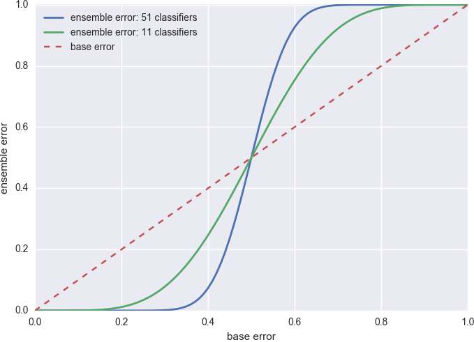
Figure 3. Error of the voting classifier.
As you can see, as long as each base classifier does better than random guess (\(\epsilon=0.5\)), the voting classifier further reduces the error. And when that happens, the more base classifiers the better.
There is one underlying assumption in this error reduction though:
- the base classifiers are not correlated
Otherwise there is no point averaging them. The fancier classifiers such as bagging, boosting, and random forest, use different ways to construct uncorrelated trees.
bagged trees
Bagging is short for bootstrap aggregating. As the name indicates, you first bootstrap then average over the results.
bootstrap
It is a resampling method that generates new dataset from original dataset following the two rules
- sample with replacement
- keep sample size the same
For example, if our dataset is two balls in an urn, one black one red, then the bootstrap sample could be (black, black), (black, red) or (red, red). Thus if we compare the bootstrap dataset to the original dataset, some data points would be excluded and some would have several copies. If we run an unstable classifier on the bootstrap dataset, we are almost guaranteed to get a somewhat different model: more uncorrelated to the original one if the classifier is more unstable.
why bagging works
Recall that in our case, bootstrap is done on the training data for fitting new decision trees. Ideally, we want to get another independent training dataset. Or even better, obtain many more independent training datasets and train a decision tree on each of them, then average over the predictions of the trees. You will probably agree that the averaged tree with extra training data would perform better than any individual tree. But why would bagging (‘fake’ extra training data) help?
First, let’s look at some fictitious plots. Let’s assume that we have three base classifiers trained with different bootstrap datasets, each of which has 80% accuracy and we average over them (majority vote). Note here I am imagining the data come from a generative model and the 80% accuracy is with respect to the generative model (or you can think of training + test data).
If the classifier is stable, the three base classifiers may agree on most data, let’s say 70% of them. In this case majority vote actually hurts! We actually end up with worse accuracy for the voting classifier, see Figure 4 for an example.
Figure 4. Voting classifier gets 70% accuracy even though the 3 base classifiers all have 80% accuracy.
On the other hand, if the classifier is unstable, the base classifiers trained on bootstrap datasets may agree on only small portion of the data, see Figure 5 for an example. This is exactly when majority vote works: the voting committee has to be both informed (better than random guess accuracy) and diverse (uncorrelated from each other).
Figure 5. Voting classifier gets 100% accuracy even though the 3 base classifiers all have 80% accuracy.
As a summary, bagging does not always work. It only works for unstable classifiers when the classifiers trained on bootstrap data do not agree too much. Thus the magic is partly in the classifiers and partly in the data itself.
One example is shown in Figure 6 where the data points follow Gaussian distributions. The two Gaussians center at (1, 1) and (3, 1) and share the same standard deviation 0.5. Ideally the decision boundary should be at \(x_1=2\). The code can be found here.
As you can see, one black dot is mingled to the white dot region and it strongly affects the decision tree result. On the other hand, the bootstrap samples may not contain this ‘outlier’ and thus provide less deviated decision boundaries. In this case, the bagged trees classifier has higher accuracy than the decision tree classifier for the test data.
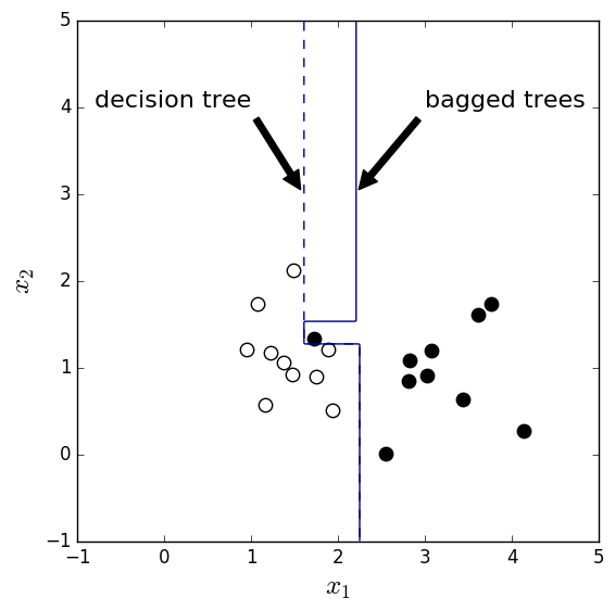
Figure 6. Decision boundary of decision tree and bagged trees classifiers for two Gaussian blobs centered at (1, 1) and (3, 1).
From this example we can conclude that if the unstable classifier is messed up by some small number of outliers, bagging should help.
random forest
Two ideas are used in the random forest classifier:
- bagging
- random feature subsets for each tree
The second idea makes the individual trees less correlated to each other. Intuitively, it should help. As for why it works well in mathematical terms, I don’t have any explanation.
boosted trees
As you have seen in Figure 4 and 5, the voting classifier works better when the base ones do not agree with each other on the same regions. The technique of boosting explicitly construct base classifiers to perform well on different data points.
The boosted trees classifier contains an iterative process to construct base classifiers. The idea is that you keep creating new classifiers that do well on the data that the old classifiers do not do well on. Typically the base classifiers are trees with depth one (also called stumps) so that data training can be less expensive.
Two weights are introduced during the iterative process
- a weight \(w_i\) at the iterative stage for focusing on the data wrongly classified in the previous rounds
- a weight \(\alpha_i\) at the voting stage for focusing on the good base classifiers
There is a magic relationship between the two weights, which can be found in books and talks. I don’t understand how it works but it seems there are some theoretical understanding about why boosted trees work.
summary
As you can see, my understanding on random forest and boosted trees is quite poor. I am not sure what the mathematical tool is to analyze their errors since the branching of decision tree is somewhat ad hoc. Two of my data scientist friends (one math PhD, one physics PhD) recommended me a book to learn machine learning in general and it indeed has quite some discussions on tree-based methods.

Unfortunately, I find this book hard to follow, maybe due to my lack of math education. If you know any good learning material on tree-based methods, especially on the error analysis, please let me know.


